

Precision Agriculture
What is Precision Agriculture?
Precision agriculture (PA) is a the practice of managing crop production inputs, e.g. seed, nutrients, ameliorants, herbicides and pesticides etc, along with GPS-based machinery control, on an in-field, site-specific basis. This will help to maintain and increase the quality of the environment, reduce waste, reduce the use of agricultural chemicals and nutrients while containing or improving farmer profits.
What are the benefits of PA?
- Potential higher yields and higher profits,
- More effect use of nutrients and chemicals and time,
- Zonal management options in relation to cultivation, soil amendment and chemical applications,Improved fatigue management (especially with autosteer systems).
What is included in PA?
Precision agriculture technologies include:
- Equipment guidance and automatic steering,
- Yield monitoring,
- Variable rate input application,
- Remote sensing, in-field electronic sensors,
- Section and row control on planters,
- Sprayers and fertilizer applicators, and
- Spatial data management systems.
What are the three main elements for PA?
Precision Agriculture (PA) is a farm management approach using information technology, satellite positioning (GNSS) data, remote sensing and proximal data gathering. These technologies have the goal of optimising returns on inputs whilst potentially reducing environmental impacts.
PA at HCPSL
HCPSL currently own and manage a free-access community GNSS (GPS, GLONASS, GALILEO, BEIDUO, QZSS) base station network in the Herbert region. This is the basis for PA in the Herbert, including control traffic and permanent crop beds within field, variable rate nutrient and ameliorant application. Many of the cane harvesters in the district also use GPS when harvesting to reduce compaction on crop beds, improved cane feeding and to manage driver fatigue.
Recently harvester manufacturers have developed yield monitors for their machinery which used GPS to monitor crop yield (tonnes per hectare) within field. Use of this information can help growers and agronomists to identify lower producing areas in cane blocks which can be managed differently to the better producing areas within the block. HCPSL’s isn’t the only GNSS network in the Herbert, John Deere have several Greenstar base stations around the district, and some growers have their own base stations installed.
HCPSL owns a DualEM 421s which collects data on the apparent electromagnetic conductivity (ECa) of the soil. EM data helps by identifying variation in the soils in a cane block. This is then used for targeted soil sampling and, along with satellite imagery, becomes the basis for VR prescription maps for ameliorants and nutrients.
HCPSL makes use of the European Space Agency’s free Sentinel 2 satellite imagery. Imagery is downloaded and analysis is undertaken using NDVI or GNDVI (normalised difference vegetation index or Green NDVI) algorithms. These indices identify health and vigour of the crop. These data can be used alongside EM data to better understand crop health and yield within a field.
Using the data described above and in consultation with the cane grower, agronomists at HCPSL, having identified infield management zones and, using soil test results, can produce VR prescriptions for ameliorants and/or nutrients for individual cane blocks. These maps are then entered into the VR controller in a tractor, and nutrient/ameliorant is applied at variable rate, as required, across the block.
Links
https://www.precisionag.com/market-watch/precision-agriculture-terms-and-definitions/
https://www.ag.ndsu.edu/agmachinery/precisionagriculture
Satellite imagery at HCPSL
Brief History
The Earth Resources Technology Satellite (ERTS-1, later renamed Landsat 1) was launched carrying two main camera systems, a Return Beam Videocon (RBV) and a Multispectral Scanner System (MSS)[1], the important one for NDVI. Initially Landsat images had a resolution of 80m which was too coarse for agricultural purposes at a farm scale or block scale. By Landsat 4 in 1982, images were acquired at a 30m resolution and were beginning to be used to look at agricultural productivity.
From the late 1990’s HCPSL gained access to LANDSAT, SPOT imagery via the HRIC (Herbert Resource Information Centre), through research driven projects and researchers such as Dr Andrew Robson among others. Much of this research centred around the development of crop yield estimates via satellite image analysis. Only in the last couple of years has this work resulted in suitable crop yield forecasting, thanks to the efforts of Dr Robson and his team.
In 2015 the European Space Agency launched the first of two satellites (Sentinel 2A and then Sentinel 2B in 2017), to measure environmental metrics across the earth. Sentinel 2A and 2B specifically, collect data which is applicable to agriculture and vegetation management. This data is provided to users at no cost to promote its use in vegetation and crop management. Data resolution is 10m for the image bands applicable to NDVI and vegetation management while others are either 20m or 60m for atmospheric composition[2].
Current Usage of Satellite Imagery
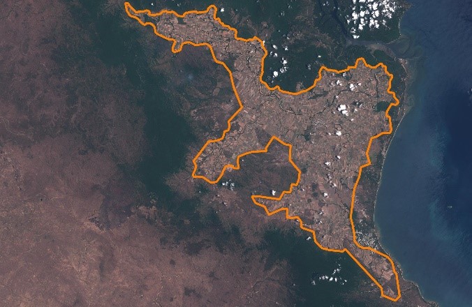
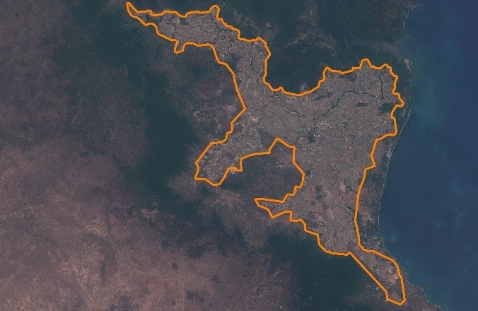
The two Sentinel 2 satellites have opposing ten-day return cycles. This means that they both acquire imagery over the same area on the earth every ten days and because there are two satellites, an image is captured every five days over the same area. In theory we should get 73 images of the district each year, one every five days. Trouble is that cloud obscures the satellite’s view of the earth and while an image is acquired every five days, many are unusable, or are only partly usable as is illustrated by the images below.
During 2019 HCPSL downloaded 72 satellite images (the 23rd of June image was not available), 43 were unusable (e.g. the 19th of January and 13th of July images), 13 were partly usable (the image still had significant cloud coverage, e.g. the 24th of May), 4 were almost clear but still had small areas of cloud (e.g. the 20th of November), and 7 were cloud free (e.g. the 13th of February and the 25th of December images).
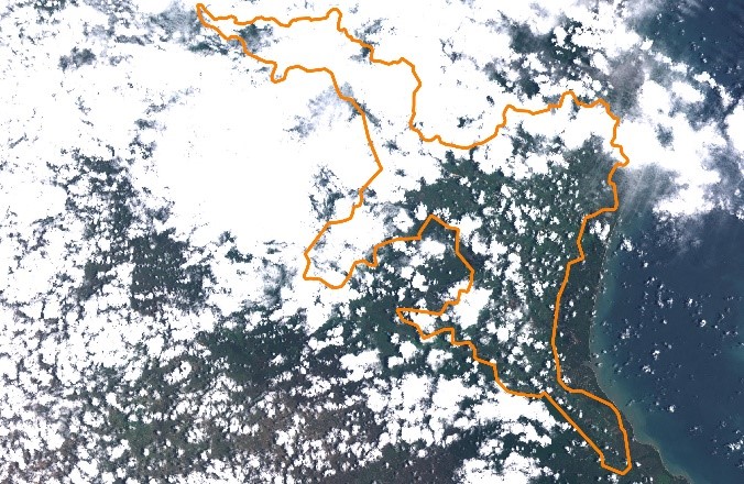
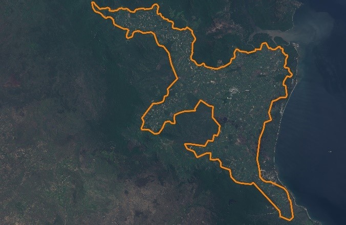
The image from the 19th of January (above) shows cloud covering the whole Herbert region. This leaves very little usable data, that is, visible ground, for analysis. The image from the 13th of February, however, shows the district cloud free. Cloud-free data like this allows the whole district to viewed and analysed using indices like NDVI. HCPSL does this analysis in-house and creates a series of maps for each farm across the district. These maps are held in-house at HCPSL and are available to growers upon request.
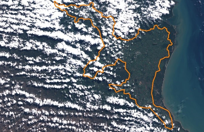
The image from the 24th of May shows part of the district cloud free, and the rest with a significant amount of cloud. Images like these are held by HCPSL but no analysis is done unless specifically requested by HCPSL staff for comparison against other data, such as EM data.
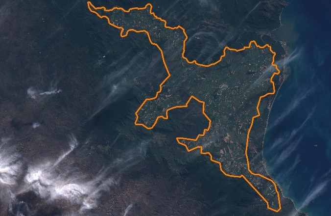
The 13th of July image shows high cloud covering much of the district which will negatively affect any analysis undertaken. Hence no analysis is done using data like this. The image from the 20th of November shows the district almost clear of cloud. This data is usually analysed using NDVI, but much care needs to be taken not to misinterpret the cloud and cloud shadow as part of the crop. The 25th of December image again is cloud-free.
Many of the farm management software packages allow satellite imagery, or their derivative products, like NDVI to be imported and used in crop performance analysis. For example, several years of available NDVI (or GNDVI) imagery can be used to determine high to low growth zones within a field. Some software allows analysis with other data such as electromagnetic induction, while other allow block productivity data to be added to produce a yield map, post-harvest. Work is also proceeding to produce accurate crop yield estimate maps using vegetation indices and historical crop productivity data.
[1] https://www.usgs.gov/land-resources/nli/landsat/landsat-1?qt-science_support_page_related_con=0#qt-science_support_page_related_con
[2] https://en.wikipedia.org/wiki/Sentinel-2
HCPSL Using NDVI.
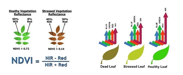
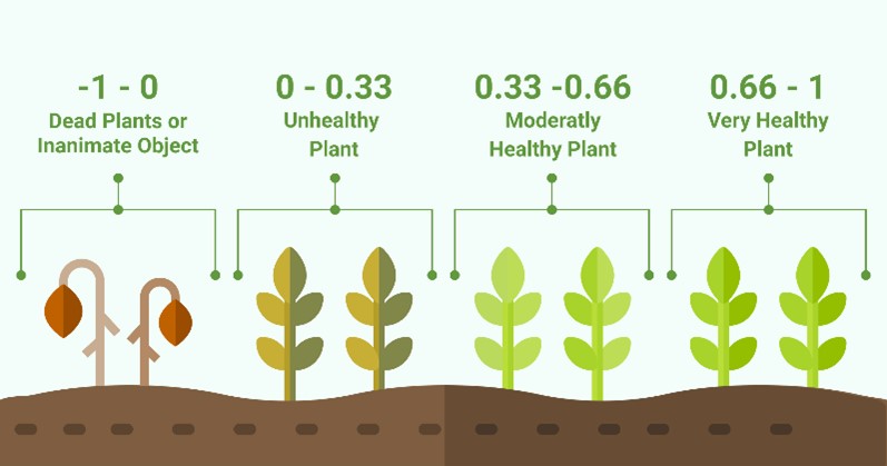
NDVI is one of the best known of the vegetation indexes which quantifies vegetation health and vigour by measuring the difference between near-infrared light (which vegetation strongly reflects) and red light (which vegetation absorbs).[1] It is yet another tool in the toolbox for farmers to quickly assess the potential productivity within a paddock.
The formula for NDVI is:
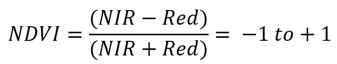
Essentially, the chlorophyll pigment in healthy plants absorbs most of the red light and blue light in the visible band (spectrum), and reflects more of the green visible band, and reflects still more of the near infrared light (NIR), one of the invisible bands. Because chlorophyll reflects more green light that either red or blue, a plant’s leaf looks green to the naked eye. The greener a leaf, usually an indicator of good plant health, means that less red light is reflected. Therefore, using a normalised ratio between the highly reflected NIR light band and the poorly reflected red light band, a scale, or index is created, which provides an indication of plant health and vigour.
https://eos.com/blog/ndvi-faq-all-you-need-to-know-about-ndvi/
The results of NDVI always range between -1 and +1 but there are no distinct boundaries between plant health classes or land cover type. However, values close to +1 usually represent healthy vegetation while values close to and below 0 are usually bare ground or water1.
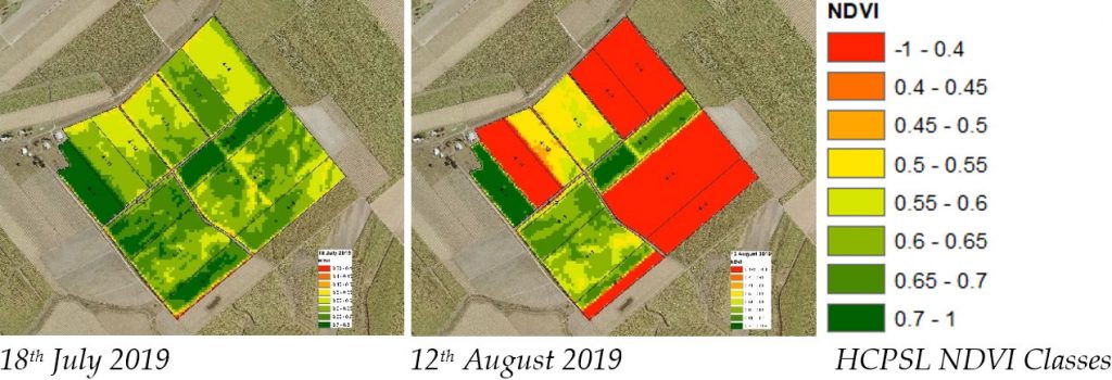
The following images show change in crop health/vigour over time. Remembering the 2018/19 extreme rainfall events, the effects can be seen in the NDVI farm maps along with the recovery of the crop over time. The final image shows the NDVI class distinctions used by HCPSL. This allows comparison between blocks on farms. HCPSL typically uses an eight class, red to green colour ramp to represent the health/vigour of the crop, red being bare ground or very sparse/poor vegetation. The transition to the darkest green indicates a crop canopy which is gradually covering any visible ground (showing primarily leaf matter) and growing vigorously. Legume crops grown as part of fallow management often show as the darkest green. As the sugarcane matures, the shade of green in the leaf tends to lighten (senescence), and this is reflected in the shade of green in the image.
Note that cane varieties which flower heavily will also affect the reflectance and therefore the NDVI values, usually showing as less vigorous. Some growers are using NDVI to interpret crop maturity, as a guide to their harvesting schedule.
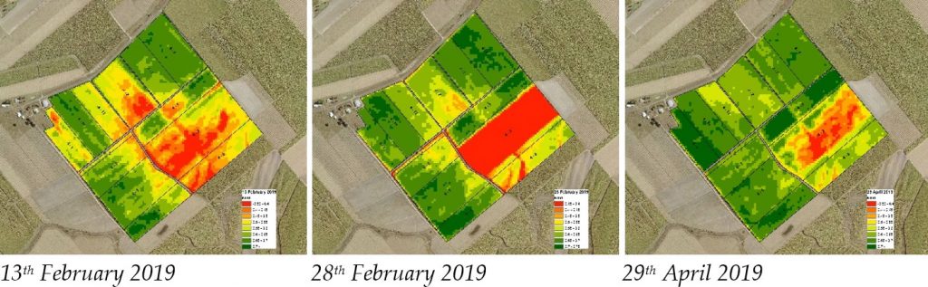
The 13th of February image shows a significant amount of crop damage due to the extreme rainfall events over the 2018/19 summer (almost three metres of rain fell over a twelve week period between the 4th of December, 2018 and the 1st of March, 2019). The 28th of February image shows some recovery in parts of the crop along with a cane block having been sprayed out as fallow (the big red rectangle). The 29th of April image shows good recovery across most of the farm and shows the fallow block still with bare ground showing.
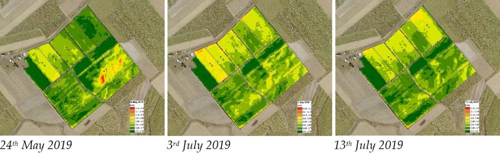
The images from the 24th of May through to the 18th of July show increasing crop vigour as the season progresses. The 12th of August image shows that several cane blocks have been harvested along with other blocks maturing. Having a mid-harvest snapshot of the crop may give reason to make changes to the harvesting schedule to try to maximise CCS.
HCPSL made use satellite imagery and NDVI over the 2018 March flood and the 2018/19 extreme wet season to find areas with significant damage from inundation. This identified areas for a closer inspection and recording using HCPSL’s drone. This also helped with the assessments undertaken by DAF for governmental assistance.
One of the advantages is the ability for farm management software packages to import NDVI imagery. Commercial companies such as DataFarming have an ability to view NDVI imagery online for free, or imagery can be downloaded at a cost, and used within farm management software packages. In other platforms like ProAgrica (SST), imagery can be purchased through associated apps and become available within the software. The limitation of many of these systems is that imagery can only be viewed by individual block. DataFarming allows the ability to create an “area of interest” polygon which can be as big as the user wants.
HCPSL downloads the Sentinel 2 imagery as it becomes available. When cloud-free images are available, NDVI analysis is performed and a district-wide set of farm maps is created and stored on HCPSL’s server. These are used by HCPSL’s agronomists and are available to growers on request.
HCPSL has started doing multi-image and where possible, multi-year analysis of NDVI imagery on a block by block basis where required. With multi-year analysis it is good to have images from around the same date each year, however sometimes this is not possible due to cloud cover. Where images are available near to the same dates, care needs to be taken due to the possible effects of nutrient application and/or rain/irrigarion.
As research into remote sensing continues, additional vegetation indices are developed for us in estimating crop health. GNDVI, or green NDVI is a modified version of the NDVI algorithm that uses Green and NIR light to better indicate the variation of chlorophyll content in the vegetation. It is also useful to analyse deficit/excess of water and nitrogen in the crop[2].
Drone-mounted multispectral cameras, after processing, can produce the same results, NDVI etc. at a much smaller resolution, good for trials and small crops.
image 1 https://www.integraldrones.com.au/comparing-ndvi-mapping-systems/
image 2 https://eos.com/blog/ndvi-faq-all-you-need-to-know-about-ndvi/
[1] https://gisgeography.com/ndvi-normalized-difference-vegetation-index/
[2] https://support.dronedeploy.com/docs/understanding-ndvi-1#:~:text=Green{d47fdfd655866cbe7bd35ef217e0cbde27d2ee6ecb2f0d5a3dfe6c4b299e6d14}20Normalized{d47fdfd655866cbe7bd35ef217e0cbde27d2ee6ecb2f0d5a3dfe6c4b299e6d14}20Difference{d47fdfd655866cbe7bd35ef217e0cbde27d2ee6ecb2f0d5a3dfe6c4b299e6d14}20Vegetation{d47fdfd655866cbe7bd35ef217e0cbde27d2ee6ecb2f0d5a3dfe6c4b299e6d14}20Index,and{d47fdfd655866cbe7bd35ef217e0cbde27d2ee6ecb2f0d5a3dfe6c4b299e6d14}20nitrogen{d47fdfd655866cbe7bd35ef217e0cbde27d2ee6ecb2f0d5a3dfe6c4b299e6d14}20in{d47fdfd655866cbe7bd35ef217e0cbde27d2ee6ecb2f0d5a3dfe6c4b299e6d14}20the{d47fdfd655866cbe7bd35ef217e0cbde27d2ee6ecb2f0d5a3dfe6c4b299e6d14}20crop.


